MOTER (Modeler of Three Energy Regimes)

MOTER is an optimization tool for the dispatch of ‘multi-commodity’ energy systems consisting of interconnected electricity, natural gas, hydrogen and heat networks. MOTER was developed in the period 2015-2020 DNV as the calculation engine for the DNV ‘Energy Transition Simulator’ (ETS). The ETS allows for 10-15 participants in a workshop setting to explore decarbonization pathways, from 2020 to 2050, for a simple fictive world (‘Enerland’), but with real world techno-economic physics and price models. As the physics engine, MOTER dispatches all production, end use, transport, conversion and storage assets of Enerland energy system at lowest overall cost. The objective of MOTER within the Multi-Model macro case is to add network dispatch and in particular network congestion management to a the national ‘II3050-Mobility’ case.

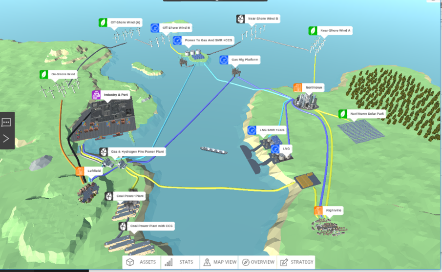
The original Enerland case in the Energy Transition Simulator.

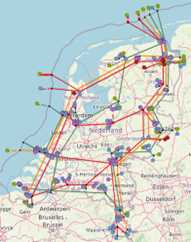
the Netherlands-II3050-Mobility network template in the MultiModel

MOTER scope

The objective of MOTER (Modeler of Three Energy Regimes) is to find the optimal techno-economic performance of an externally provided multi-commodity energy system, consisting of the topology and capacities of following assets:

• Primary energy generation via wind turbines, solar PV, geothermal, coal power plants (+CCS), natural gas production and energy import/ export.

• Residential, industrial heat &power demand centers via ‘smart’ end use applications.

• Energy conversion via gas-to-power, power-to-gas, power-to-heat, gas-to-heat, natural gas to hydrogen technologies.

• Energy transport networks consisting of power cables, gas pipelines, heat networks (+ transformers, compressors)

• Energy storages (battery, pumped hydro, underground gas storage, insulated hot water tanks)

The output of MOTER is the cost optimal ‘dispatch’ of the flex in the energy system. The term ‘flex’ refers to any measure the market can take to reduce supply-demand imbalances, such as:

• Bridging energy supply-demand imbalances in space using passive assets (pipes and cables) in combination with dispatchable assets (compressors and transformers)

• Bridging energy supply-demand imbalances in time using storage.

• Bridging energy supply-demand imbalances in energy type using conversion.

Additional ‘flex’ options:

• Production flex: Ramp-up of flexible sources (natural gas, oil import etc.), curtailment of fixed sources (solar PV, wind turbines, geothermal, etc) according to relative merit orders.

• End user flex: Curtailment and time shifting of energy end use according to relative merit orders (industrial/ residential v. electric power/ space heating).

• Conversion flex: multi-fuel operations (heat pump+ natural gas back up)

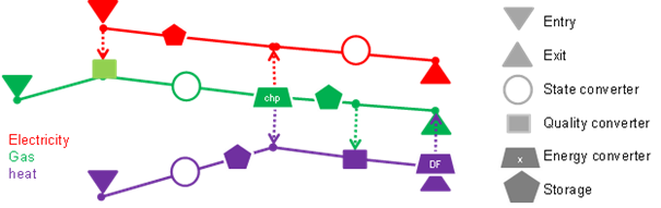
Illustration of a multi-commodity energy system in MOTER. Energy carriers enter the system via network ‘entries’ (producers) and leave via network ‘exits’ (consumers). To match supply -demand, energy carriers can transported via cables pipes and stored in storages. Energy carriers can be converted from carrier A -> B via (energy) converters (boilers, electrolyzers, steam methane reformers), Energy ‘states’ (voltage, prerssure) can be altered using (state) converters like compression/ transformers. The ‘quality’ of the energy (mainly gas calorific value, heat network water temperature) can be changes via (quality) converters like natural gas to hydrogen converters, gas mixing stations and back-up heaters. MOTER does not yet model AC power ‘cos phi’ or reactive power.

Energy carriers in scope are:

Energy carriers	Subtypes	Modeled properties
electricity	HV, MV, LV	Voltage, current (DC eq.), power
EGaseous	Natural gas , biogas, hydrogen	Pressure, flow, Calorific value, power
Heated water	Heat network, local demand	Pressure, flow, temperature, power
External fuels	Oil, coal, nuclear	Flow, Calorific value, power

The assets in scope are:

Type	Examples	Input parameters	Output
Production/entries	Wind turbine, gas field, geothermal, oil import	Capacity, curtailment / import cost, requested profile	Operational hours, realized profile
End use/ exits	Industrial/ residential, Heat/ power, mobility	Capacity, curtailment / export cost, requested profile	Operational hours, realized profile
Converter (carrier)	Gas-to-power, power-to-gas, gas-to-heat, power-to-heat, natural gas to hydrogen	Capacity, efficiency	Operational hours, realized profile
Converter (transport)	Transformer, compressor	Capacity, efficiency	Operational hours, realized profile
Converter (quality)	Gas blending, heat booster	Capacity, efficiency	Operational hours, realized profile
Transport	Cable, pipe	Length, conductivity	Operational hours, realized profile
Storage	Battery, salt cavern, hot water tank	Volume, send-in/out capacity	Operational hours, realized profile

Special feature: time slices

A special challenge when working with optimization modeling is the maximum number of assets that can be modelled in combination with properties and time resolution. In other words, the size of the ‘objects(variables,T) matrix’ that will still fit into computer memory and can be solved in acceptable calculation. Macro Energy modelling requires that both the seasonal and the intraday dynamics must be captured by the model. However modeling 8760 hours/year will ‘blow up’ memory usage and severely restricts the number of active objects (distributed and connected in space and including subcategories) that it becomes unsuitability for real world applications. This especially when Monte Carlo methods (‘perform a great number of runs with stochastically varied inputs’) are being considered and model runs need to be (very) fast. The solution in MOTER, as is used for Opera, is to reduce the 8760 hours to a define a subset of ‘time slices’ during the year. This because a series of 8760 hours will contain a significant amount of redundant information. In one case study and it was established that with only 16 snapshots (night/morning/afternoon/ evening & winter, spring, summer, autumn) sufficient accuracy (~>90%) may already be achieved, in only a fraction ( <1%) of the calculation time. In order to create a 8760 hour profile from the snap shots a simple ‘sample & hold’ reconstruction algorithm is used.

Note that when using ‘global optimization’, special care has been taken is that the relative order of the snapshots, i.e. causality, is being respected. This because global optimizers calculate all time steps all at once, unlike simulators which run though time step consequently. MOTER has extra time hierarchy information on first priority on the intraday snapshot order first (night, morning, afternoon, evening) and then the days ordering during the year next (jan 1st –> December 31st). This ‘proper time ordering’ is important when optimizing energy storage systems that perform both intraday and seasonal balancing functions.

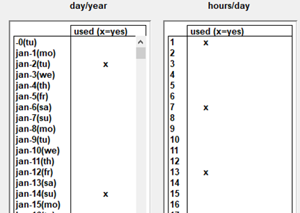
Example of defining the time slices that serve as ‘proxies’ for the reconstruction of full year dynamics.

For more information see Netbeheer Nederland datasheet about MOTER

Additional documentation

Note that more documentation about MOTER on the TU-Delft server can be found under AIMMS_models